LightWin compensation example
This notebook showcases how to compensate for a single failure.
Imports
Note that the first import is only used to import packaged data file. See also: https://learn.scientific-python.org/development/patterns/data-files/
[1]:
from importlib import resources
from pprint import pprint

# Actual mandatory imports for LightWin
from lightwin.config.config_manager import process_config
from lightwin.ui.workflow_setup import run_simulation
Presentation of the linac
The structure of the linac is stored in a DAT file. It follows the same specifications as TraceWin structure file, see associated help page for more information. The example can be found in data/ads/ads.dat (or src/lightwin/data/ads/ads.dat if you built LightWin from source). Here are the first lines of the file:
[2]:
dat_res = resources.files("lightwin.data.ads") / "ads.dat"
dat_content = dat_res.read_text(encoding="utf-8")
print(dat_content[:892])
;------------------------------------
; TraceWin Version: 2.23.1.3
; OS: Win10 (64-bit)
; Date: Fri Oct 20 14:31:57 2023
; User: FBOULY
; Computer: LPSC5003W
;------------------------------------

FIELD_MAP_PATH field_maps_1D


; Section #1

LATTICE 10 0
FREQ 352.2
; Lattice #1
QUAD 200 5.66763 100 0 0 0 0 0 0
DRIFT 150 100 0 0 0
QUAD 200 -5.67474 100 0 0 0 0 0 0
DRIFT 150 100 0 0 0
DRIFT 589.42 30 0 0 0
FIELD_MAP 100 415.16 153.171 30 0 1.55425 0 0 Simple_Spoke_1D 0
DRIFT 264.84 30 0 0 0
FIELD_MAP 100 415.16 156.892 30 0 1.55425 0 0 Simple_Spoke_1D 0
DRIFT 505.42 30 0 0 0
DRIFT 150 100 0 0 0
; Lattice #2
QUAD 200 5.77341 100 0 0 0 0 0 0
DRIFT 150 100 0 0 0
QUAD 200 -5.77854 100 0 0 0 0 0 0
DRIFT 150 100 0 0 0
DRIFT 589.42 30 0 0 0
FIELD_MAP 100 415.16 161.635 30 0 1.56423 0 0 Simple_Spoke_1D 0
DRIFT 264.84 30 0 0 0
FIELD_MAP 100 415.16 165.455 30 0 1.56423 0 0 Simple_Spoke_1D 0
This is a high-power, ADS-like proton acceleractor characterized by a very high longitudinal acceptance.
Configuration of LightWin
In order to ensure reproducibility and portability of results, all the configuration is set in a TOML configuration. The full specifications are listed in Configuration.
[3]:
toml_filepath = resources.files("lightwin.data.ads") / "lightwin.toml" # Or provide Path to TOML file
Below, we associate LightWin’s configuration objects with sections in the TOML file (the names between brackets).
[4]:
toml_keys = {
    "files": "files",
    "beam": "beam",
    "beam_calculator": "generic_envelope1d",
    "wtf": "generic_wtf",
    "design_space": "fit_phi_s_design_space",
    "plots": "plots_minimal",
}
This operation will check validity of the configuration, resolve paths, and convert the TOML appropriate entries to a dictionary.
[5]:
# Adapt some configuration entries for this notebook
override = {
    "beam_calculator": {
        "flag_cython": True,  # Override flag_cython=False in [generic_envelope1d]
    },
    "wtf": {
        "k": 5,               # Override k=3 in [generic_wtf]
    },
    "plots": {
        "kwargs":
        {
            "lw": 5,          # Increase size of lines in plots
        },
    },
}
config = process_config(toml_filepath, toml_keys, override=override)
[INFO    ] [log_manager.py      ] Starting log for LightWin - Version: 0.16.3.dev1+g4c96aaf, Commit: 4c96aaf2a12e1dbfd514865321331c13ad57cc82
[INFO    ] [files_specs.py      ] Setting project_path = PosixPath('/home/docs/checkouts/readthedocs.org/user_builds/lightwin/envs/latest/lib/python3.12/site-packages/lightwin/data/ads/lw_results')
Setting log_file = 'lightwin.log'
files (doc)
Defines the files to use, as well as where results should be saved.
[6]:
pprint(config["files"])
{'dat_file': PosixPath('/home/docs/checkouts/readthedocs.org/user_builds/lightwin/envs/latest/lib/python3.12/site-packages/lightwin/data/ads/ads.dat'),
 'project_folder': PosixPath('/home/docs/checkouts/readthedocs.org/user_builds/lightwin/envs/latest/lib/python3.12/site-packages/lightwin/data/ads/lw_results')}
beam (doc)
Define the beam properties.
[7]:
pprint(config["beam"])
{'e_mev': 20.0,
 'e_rest_mev': 938.27203,
 'f_bunch_mhz': 100.0,
 'gamma_init': 1.021315779817075,
 'i_milli_a': 0.0,
 'inv_e_rest_mev': 0.0010657889908537506,
 'lambda_bunch': 2997924.58,
 'm_over_q': 938.27203,
 'omega_0_bunch': 628318530.7179586,
 'q_adim': 1.0,
 'q_over_m': 0.0010657889908537506,
 'sigma': array([[ 8.409896e-06,  3.548736e-06,  0.000000e+00,  0.000000e+00,
         0.000000e+00,  0.000000e+00],
       [ 3.548736e-06,  1.607857e-06,  0.000000e+00,  0.000000e+00,
         0.000000e+00,  0.000000e+00],
       [ 0.000000e+00,  0.000000e+00,  2.941564e-06,  6.094860e-07,
         0.000000e+00,  0.000000e+00],
       [ 0.000000e+00,  0.000000e+00,  6.094860e-07,  4.418911e-07,
         0.000000e+00,  0.000000e+00],
       [ 0.000000e+00,  0.000000e+00,  0.000000e+00,  0.000000e+00,
         3.593136e-06, -2.552518e-07],
       [ 0.000000e+00,  0.000000e+00,  0.000000e+00,  0.000000e+00,
        -2.552518e-07,  5.994771e-07]])}
beam_calculator(doc)
Define how the propagation of the beam in the linac will be calculated. Note that you can define a beam_calculator_post in a similar fashion; it will be used to re-compute the propagation of the beam once the compensation settings are found.
[8]:
pprint(config["beam_calculator"])
{'export_phase': 'phi_0_abs',
 'flag_cython': True,
 'method': 'RK4',
 'n_steps_per_cell': 40,
 'reference_phase_policy': 'phi_0_abs',
 'tool': 'Envelope1D'}
Some comments on the settings we chose:
Envelope1Dis usually a good choice, as transverse dynamics are not very important for failure compensation.n_steps_per_cell=40withmethod="RK4"are a good balance between precision and rapidity.export_phase="phi_0_abs"andreference_phase_policy="phi_0_abs"to avoid implicit rephasing of the linac. See also: dedicated notebook.flag_cython=Trueto speed up the calculations. The speed-up factor is 2 to 4 on my machine. See also documentation.
plots (doc)
Define the plots to create at the end of the simulation.
[9]:
pprint(config["plots"])
{'add_objectives': True,
 'cav': True,
 'emittance': False,
 'energy': True,
 'envelopes': False,
 'kwargs': {'lw': 5},
 'phase': True,
 'transfer_matrices': False,
 'twiss': True}
wtf (doc)
Stands for “what to fit”.
[10]:
pprint(config["wtf"])
{'failed': [['FM11']],
 'id_nature': 'name',
 'k': 5,
 'objective_preset': 'EnergyPhaseMismatch',
 'optimisation_algorithm': 'downhill_simplex',
 'optimisation_algorithm_kwargs': {'options': {'adaptive': True,
                                               'disp': False}},
 'strategy': 'k out of n'}
failed=[["FM11"]]andid_nature="name"define one fault scenario, with one failed cavity which name is “FM11”.We try to follow TraceWin naming conventions.
strategy="k out of n"withk=5to compensate every failed cavity with the five closest cavities. The compensation strategies are defined in thestrategymodule.We overrode
k=3from originallightwin.tomlfile. The optimization process will take more time, but three compensating cavities are not enough to retrieve a perfect beam.
objective_preset="EnergyPhaseMismatch"defines three objectives to minimize: energy and phase difference with nominal linac at the end of the last compensating cavity and longitudinal mismatch factor. The objectives are defined in theobjective.factorymodule.optimisation_algorithm="downhill_simplex"to useDownhillSimplexoptimization algorithm.Note that you can provide keyword arguments to personalize the execution of the algorithm.
Downhill simplex is very fast and effective for this kind of problem, with few variables.
design_space (doc)
Defines the design space, i.e. the optimization variables and their bounds.
[11]:
pprint(config["design_space"])
{'design_space_preset': 'sync_phase_amplitude',
 'from_file': False,
 'max_absolute_sync_phase_in_deg': 0.0,
 'max_decrease_k_e_in_percent': 20.0,
 'max_increase_k_e_in_percent': 180.0,
 'max_increase_sync_phase_in_percent': 40.0,
 'maximum_k_e_is_calculated_wrt_maximum_k_e_of_section': True,
 'min_absolute_sync_phase_in_deg': -90.0}
With design_space_preset="sync_phase_amplitude", the variables will be the synchronous phase and the field amplitude of every cavity.
This generally works well with optimization algorithm that do not support constraints such as DownhillSimplex, because it allows one to bound the synchronous phase even without constraints.
See also design_space.factory for the various design space presets.
Note
You can provide a file to define different amplitude/synchronous phase bounds for every cavity. This is particularly useful for real-life problems, where every cavity has it’s own history and behavior.
Actual usage
The following function will break and fix the linac. Check out the source code of the workflow_setup module if you want to understand and personnalize this workflow.
[12]:
config["plots"]["kwargs"] = {"lw": 10}
[13]:
fault_scenarios = run_simulation(config)
[INFO ] [factory.py ] Creating new BeamCalculatorsFactory instance.
[WARNING ] [field_factory.py ] Field objects do not handle Cython yet. Will disregard cythonloading.
[INFO ] [factory.py ] Creating new BeamCalculator: 0_CyEnvelope1D
[INFO ] [accelerator.py ] Created a ListOfElements ecompassing all linac. Created with:
dat_file = PosixPath('/home/docs/checkouts/readthedocs.org/user_builds/lightwin/envs/latest/lib/python3.12/site-packages/lightwin/data/ads/ads.dat')
w_kin_in = 20.00 MeV
phi_abs_in = 0.00 rad
[INFO ] [factory.py ] Created 000000_Reference Accelerator.
[INFO ] [accelerator.py ] Created a ListOfElements ecompassing all linac. Created with:
dat_file = PosixPath('/home/docs/checkouts/readthedocs.org/user_builds/lightwin/envs/latest/lib/python3.12/site-packages/lightwin/data/ads/ads.dat')
w_kin_in = 20.00 MeV
phi_abs_in = 0.00 rad
[INFO ] [factory.py ] Created 000001_Solution Accelerator.
[INFO ] [beam_calculator.py ] Elapsed time in beam calculation: 0:00:00.261995
[INFO ] [beam_calculator.py ] Elapsed time in beam calculation: 0:00:00.249468
[WARNING ] [objective.py ] key = 'to_deg' is recommended to avoid undetermined behavior but was not found.
Objective(name=$M_{z\delta}$, weight=1.0, get_key=twiss, get_kwargs={'elt': Drift # 91 | DRIFT 150 100 0 0 0, 'pos': 'out', 'to_numpy': True, 'phase_space_name': 'zdelta'}, ideal_value=0.0, descriptor=Minimize mismatch factor in the [z-delta] plane.)
[INFO ] [fault_scenario.py ] Created a ListOfElements ecompassing a linac subset.
Encompasses: FM8 to DR42
w_kin_in = 23.00 MeV
phi_abs_in = 110.84 rad
[INFO ] [fault.py ] Starting resolution of optimization problem defined by:
====================================================================================================
Variable | Element | x_0 | Lower lim | Upper lim
----------------------------------------------------------------------------------------------------
$\phi_s$ [deg] | FM10 | -41.965 | -90.000 | -25.179
$\phi_s$ [deg] | FM12 | -41.305 | -90.000 | -24.783
$\phi_s$ [deg] | FM9 | -41.751 | -90.000 | -25.050
$\phi_s$ [deg] | FM13 | -40.409 | -90.000 | -24.245
$\phi_s$ [deg] | FM8 | -42.590 | -90.000 | -25.554
$k_e$ [1] | FM10 | 1.649 | 1.319 | 4.933
$k_e$ [1] | FM12 | 1.698 | 1.359 | 4.933
$k_e$ [1] | FM9 | 1.649 | 1.319 | 4.933
$k_e$ [1] | FM13 | 1.762 | 1.409 | 4.933
$k_e$ [1] | FM8 | 1.611 | 1.288 | 4.933
====================================================================================================
====================================================================================================
Constraint | Element | x_0 | Lower lim | Upper lim
----------------------------------------------------------------------------------------------------
====================================================================================================
====================================================================================================
Objective | wgt. | ideal value
----------------------------------------------------------------------------------------------------
w_kin @elt DR42 (out) | 1.0 | +2.70893353168837e+01
phi_abs @elt DR42 (out) | 1.0 | +2.05483843906372e+02
twiss @elt DR42 (out) | 1.0 | +0.00000000000000e+00
====================================================================================================
[INFO ] [fault.py ] Finished! Solving this problem took 0:00:10.615064. Results are:
====================================================================================================
Objective | wgt. | ideal value | final residuals
----------------------------------------------------------------------------------------------------
w_kin @elt DR42 (out) | 1.0 | +2.70893353168837e+01 | +1.28670398424902e-05
phi_abs @elt DR42 (out) | 1.0 | +2.05483843906372e+02 | +9.38482534706964e-06
twiss @elt DR42 (out) | 1.0 | +0.00000000000000e+00 | +1.17929712677434e-05
====================================================================================================
Additional info: DownhillSimplex
Optimization terminated successfully.
[INFO ] [fault_scenario.py ] Retuned cavities:
====================================================================================================
name status k_e phi_0_abs phi_0_rel v_cav_mv phi_s
0 FM8 compensate (in progress) 1.648655 135.051327 182.027899 0.696105 -43.742784
1 FM9 compensate (in progress) 1.774466 281.882764 197.793826 0.775295 -32.458857
2 FM10 compensate (in progress) 1.763047 62.205985 196.498848 0.795048 -38.921376
3 FM11 failed 0.000000 289.337404 179.090454 NaN NaN
4 FM12 compensate (in progress) 2.367101 115.407233 201.390455 1.102371 -38.806783
5 FM13 compensate (in progress) 1.837350 88.328684 219.763543 0.891349 -27.157820
====================================================================================================
[INFO ] [fault_scenario.py ] Solving all the optimization problems took 0:00:10.886989
[INFO ] [list_of_simulation_output_evaluators.py]
====================================================================================================
Fit quality:(FIXME: settings in FaultScenario, not config_manager)
----------------------------------------------------------------------------------------------------
end comp zone (DR42) end linac RMS [usual units]
$W_{kin}$ [MeV] -0.000% 0.000% 0.000
Beam phase [rad] 0.000% 0.000% 0.000
Norm. $\sigma_\phi$ @ $1\sigma$ [rad] 0.001% 0.002% 0.000
Norm. $\sigma_\phi$ @ $1\sigma$ [MeV] -0.001% -0.002% 0.000
Norm. $\epsilon_{\phi W}$ [$\pi$.rad.MeV] -0.000% -0.000% 0.000
$M_{z\delta}$ 0.000 0.000 nan
====================================================================================================
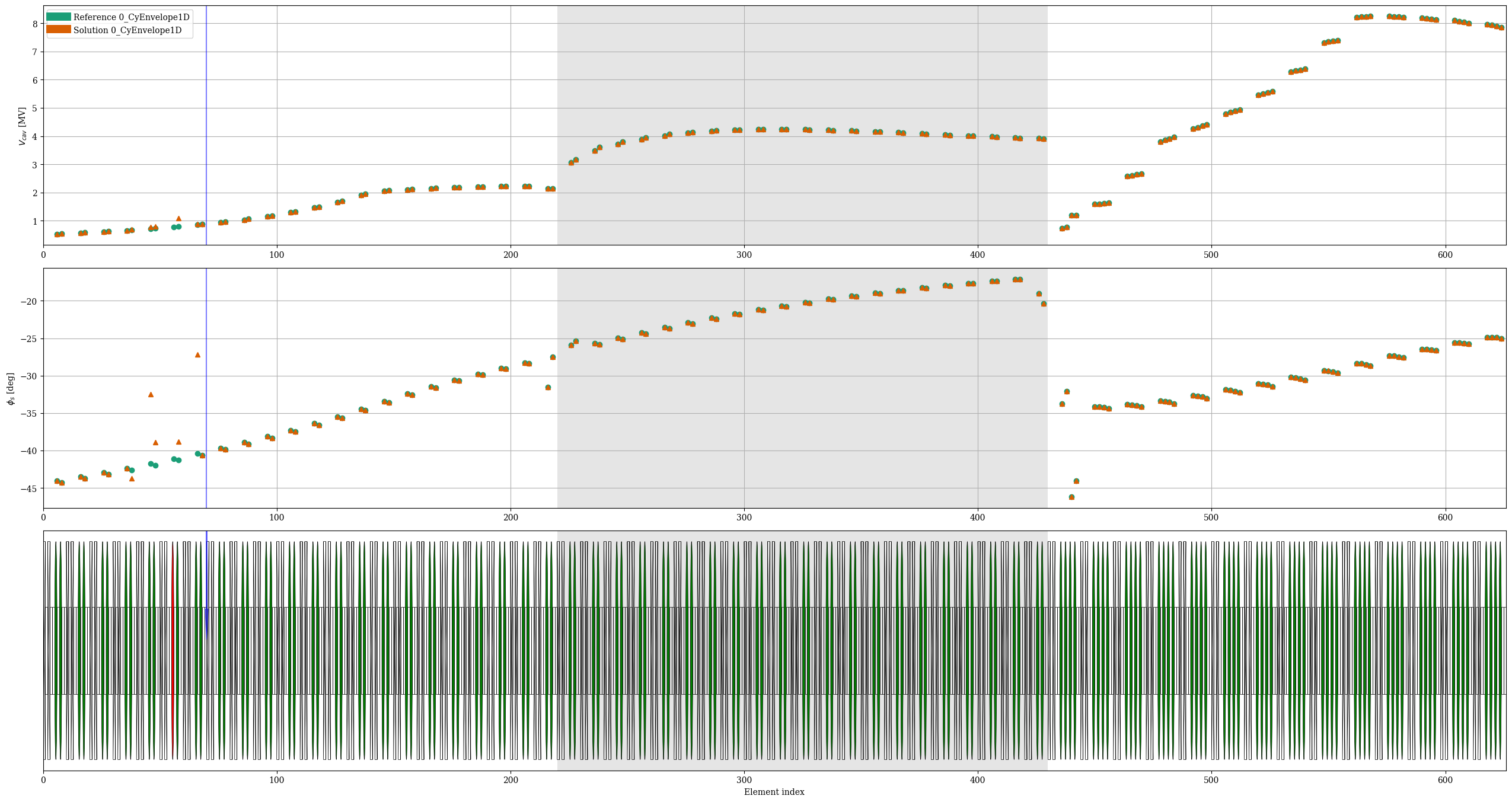
[WARNING ] [optimization.py ] When several fault scenarios are plotted after each other, they all keep the same objective position marker. This is not intended behavior.
Todo
Better display of Figures in HTML documentation.
Notes on objects hierarchy
The unique FaultScenario we studied can be accessed via:
[14]:
fault_scenario = fault_scenarios[0]
It holds two Accelerator objects, each containing a ListOfElements.
[15]:
reference_accelerator = fault_scenario.ref_acc
reference_elts = reference_accelerator.elts
[16]:
fixed_accelerator = fault_scenario.fix_acc
fixed_elts = fixed_accelerator.elts
The results are stored in a SimulationOutput object.
These latter objects are stored in a dictionary, which keys are the name of the BeamCalculator that were used.
In this case, we should only have "CyEnvelope1D_0".
A second simulation with the TraceWin solver would add a second SimulationOutput; corresponding key would be named "TraceWin_1".
The number at the end of the name represents the order in which the BeamCalculator were defined.
[17]:
fixed_simulation_outputs = fixed_accelerator.simulation_outputs
pprint(fixed_simulation_outputs)
{'0_CyEnvelope1D': SimulationOutput:
        z_abs            +0.00000e+00 -> +2.45598e+02 | (20245,)
        ParticleFullTrajectory:
                w_kin            +2.00000e+01 -> +5.02242e+02 | (20245,)
                phi_abs          +0.00000e+00 -> +1.19573e+03 | (20245,)
        BeamParameters:
                Phase space phiw:
                        alpha            -1.76610e-01 -> +1.78597e-01 | (20245,)
                        beta             +3.71099e+01 -> +6.73786e-01 | (20245,)
                        eps              +3.38012e-02 -> +3.37897e-02 | (20245,)
                        envelope_pos     +1.11998e+00 -> +1.50888e-01 | (20245,)
                        envelope_energy  +3.06472e-02 -> +2.27483e-01 | (20245,)
                        mismatch_factor   (not set)
                Phase space z:
                        alpha            +1.76610e-01 -> -1.78597e-01 | (20245,)
                        beta             +2.59322e+00 -> +8.32309e+00 | (20245,)
                        eps              +3.00000e-01 -> +2.99898e-01 | (20245,)
                        envelope_pos     +1.93596e+00 -> +1.46378e+00 | (20245,)
                        envelope_energy  +7.58100e-01 -> +1.78653e-01 | (20245,)
                        mismatch_factor   (not set)
                Phase space zdelta:
                        alpha            +1.76610e-01 -> -1.78597e-01 | (20245,)
                        beta             +2.48611e+01 -> +3.53108e+01 | (20245,)
                        eps              +3.00000e-02 -> +2.99898e-02 | (20245,)
                        envelope_pos     +1.89556e+00 -> +9.53428e-01 | (20245,)
                        envelope_energy  +7.74259e-02 -> +2.74283e-02 | (20245,)
                        mismatch_factor  +0.00000e+00 -> +1.90749e-05 | (20245,)
}
[18]:
solver_name = list(fixed_simulation_outputs.keys())[0]
fixed_simulation_output = fixed_simulation_outputs[solver_name]
Accessing data
The easiest way to access the calculated data is to use the get method.
[19]:
fixed_simulation_output.get("w_kin")
[19]:
array([ 20.       ,  20.       ,  20.       , ..., 502.2415884,
       502.2415884, 502.2415884], shape=(20245,))
[20]:
fixed_simulation_output.get("phi_s", to_deg=True, elt="FM53")
[20]:
array(-23.56086376)
[21]:
fixed_simulation_output.get("beta", phase_space_name="phiw")
[21]:
array([0.20323928, 0.20323928, 0.20323928, ..., 0.75878131, 0.75878131,
       0.75878131], shape=(20245,))
[22]:
fixed_simulation_output.get("envelope_energy_zdelta", elt="FM48", pos="out", to_numpy=False)
[22]:
np.float64(0.052032484403078436)
Note
In most case, you will want to use SimulationOutput.get() method over Accelerator.get() or ListOfElements.get(), as stated in the message below.
[23]:
fixed_accelerator.get("beta", phase_space_name="phiw")
[WARNING ] [accelerator.py ] key = 'beta': use `SimulationOutput.get()` for simulation-related attributes. `Accelerator.get()` may be ambiguous when multiple outputs exist.
[23]:
array([0.20323928, 0.20323928, 0.20323928, ..., 0.75878131, 0.75878131,
       0.75878131], shape=(20245,))